
Sometimes your data in Excel can appear as duplicates, therefore it is important to find and remove duplicate data in Excel so you can keep your worksheet organized and avoid complications.
Microsoft Excel provides lots of built-in functions and tools to make it easy to identify and manage duplicate values. In this article we will highlight ways on how to find duplicates in Excel and keep your worksheet organized.
How to Find Duplicates in Excel
There are different methods you can use to find duplicates in an Excel sheet, as well as functions that make it easy to find and remove duplicate data.
1. Use Conditional Formatting
- First select the range of cells where you want to find the duplicates. you can select a single column or row, multiple columns or rows, or an entire worksheet.
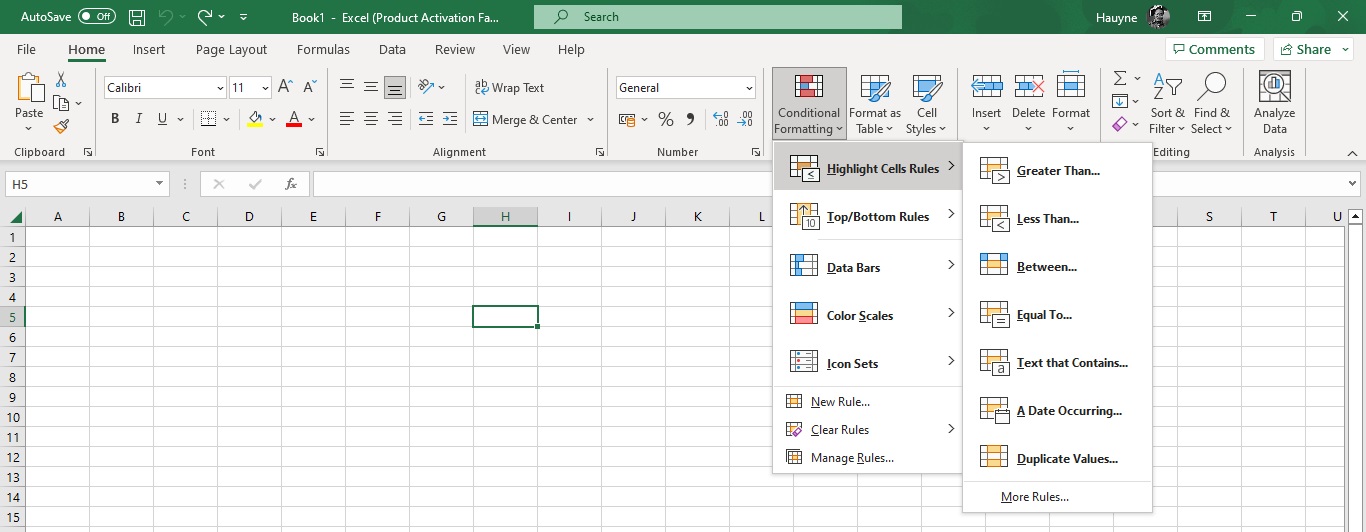
- Then proceed to open the “Conditional Formatting” menu by navigating to the “Home” tab in the Styles group, click “Conditional Formatting” .
- A drop-down menu will appear, select “Highlight Cell Rules” which is the first entry in the drop down menu.
- Then scroll down to the drop down menu that appears and select “Duplicate values”.
- The Duplicate values dialog box will appear prompting you to select how you want Excel to highlight the duplicates. There is a default format you can pick or select a different format that stands out in your worksheet.
- Click OK after making the selection.
Excel will highlight the duplicate values within the range you selected and you can easily identify them. You can click on “Unique’’ from the first drop-down list to highlight the unique data.
2. Use the COUNTIF function
Another to find and remove duplicates in Excel is to use the COUNTIF function. Using the COUNTIF function is one easy way to detect duplicates in Excel; Follow the steps below to use the COUNTIF function.
- If I have a table tagged A, B, and C where I want to find duplicates. To use the COUNTIF function, I will first create a new column and insert it next to the column I want to remove its duplicates. The new column displays the count of each value(that is the result of duplicates), the new column is named COUNT.
- In the first cell of the new column, I will combine the columns A, B, and C using the concatenation operator “&“. The Excel formula would be thus : =A2&B2&C2
- This formula is entered into a new cell D2 and then copied down to all the columns; =A2&B2&C2.
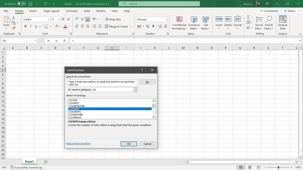
- Now I will use the COUNTIF function. The formula will be: =COUNTIF($D$2:D2,D2).
- This formula counts the number of occurrences of each value in column D.
- Drag the formula down by dragging the fill handle of the cell with the formula down to cover the entire range of cells you want to check. Excel will automatically update the cell references in the formula.
- In the new column, any values with a count greater than 1 indicates a duplicate. Sort or filter the column to bring the duplicates to the top for easy identification.
3. Use the Remove Duplicates Feature
There is a “Remove duplicates feature” one can use to find and highlight duplicate values in Excel, execute the following steps to use it.
- Select the range of cells you want to find duplicates. For example in my Excel worksheet, I will select the range A1:B10.
- Go to the Data tab in the Excel ribbon.
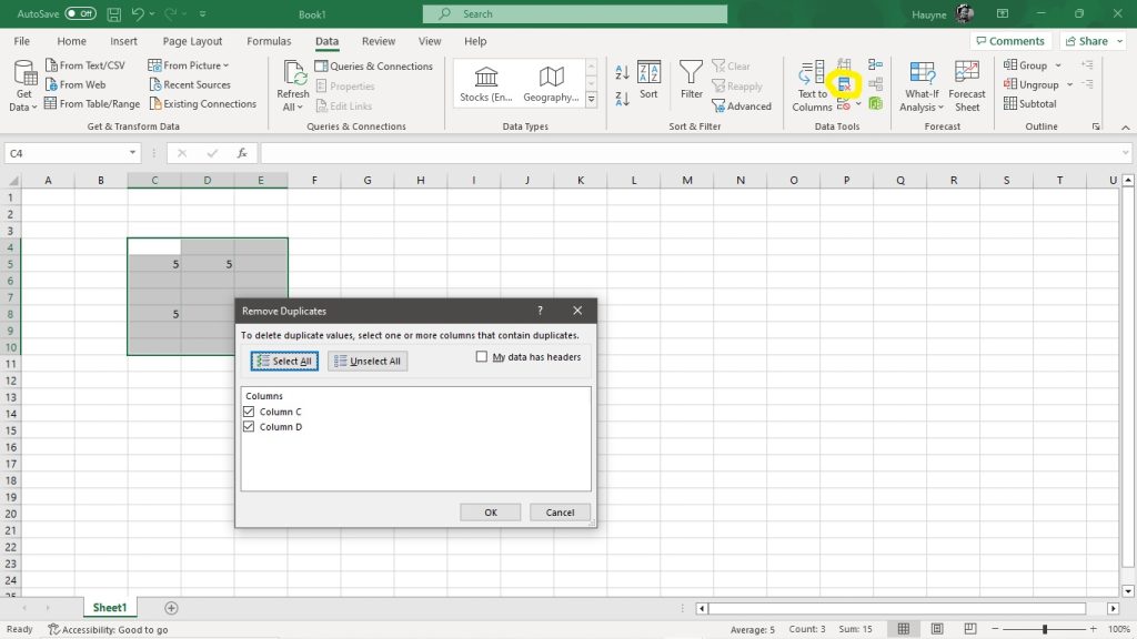
- Then click on the “Remove Duplicates” button.
- A new dialog box will open with the selected range.
- In the dialog box, choose the columns that Excel should consider when identifying duplicates. By default all columns in the selected range are included, but the selection can be customised according to a user’s needs.
- You have two options in the Remove Duplicates dialog box. “Remove Duplicates” and “Highlight Duplicates” option; select the option you want. The former will delete all duplicates and leave out the original. The latter will only highlight the duplicate values within the range.
- Once you make the selections, click OK.
Following the steps above will help you successfully find and remove duplicates in your Excel worksheet and keep your worksheet organized.